Plotting with GaussianProcesses.jl

GaussianProcesses.jl provides recipes for plotting one and two-dimensional gaussian processes using the Plots.jl package. Plots.jl provides a general interface for plotting with several different backends including PyPlot, Plotly and GR.

Currently plotting is only supported for GPE objects i.e. Gaussian processes with Gaussian likelihood functions.

Plots.jl is not a dependency of GaussianProcesses.jl as the plotting functionality is implemented through the skeleton package RecipesBase.jl. To plot a GP object one must therefore first install and load the Plots.jl package:

using Plots
pyplot()   # Optionally select a plotting backend

Plots.PyPlotBackend()

Plotting backends such as PyPlot.jl, may also have to be installed manually.

Once a GPE object is constructed, the plot command can be used to plot the mean function of the Gaussian process. The user can modify attributes of the plot such as the axis labels with the usual optional keyword arguments:

using GaussianProcesses

# Generate random data for Gaussian process
x = 2π * rand(10)
y = sin.(x) + 0.5*rand(10)

# Set-up mean and kernel
se = SE(0.0, 0.0)
m = MeanZero()

# Construct and plot GP
gp = GP(x,y,m,se)
plot(gp;  xlabel="gp.x", ylabel="gp.y", title="Gaussian process", legend=false, fmt=:png)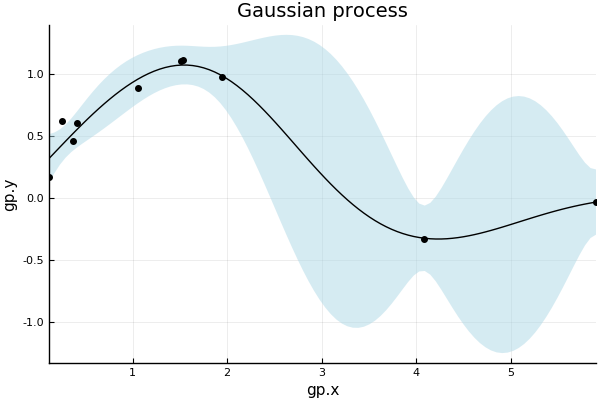

png

By default, the plot command plots the with a ribbon representing 95% confidence interval on the output observations, and with the observation points. These aspects be controlled with the following special additional keyword arguments:

β (default=0.95) : level of confidence band plotted with mean (set to 0.0 for no band)
obsv (default=true) : plot observations with mean function

Note that not all plotting backends are able to plot the confidence band. Specifically, only those which support the ribbon attribute can plot the confidence band. See here for tables detailing which backends support which series types and attributes.

Plots.jl allows the user to modify and combine plots in complicated ways. The following plots a fitted Gaussian process with sampled processes.

x = 0:0.1:2π
plot(gp; obsv=false)
optimize!(gp)
plot(gp; obsv=false, label="GP posterior mean", fmt=:png)
samples = rand(gp, x, 5)
plot!(x, samples)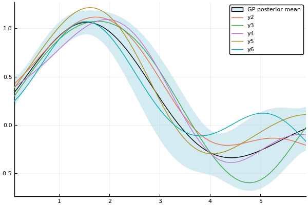

png

Two-dimensional Gaussian processes are plotted in the same way. In this case, the plot command has the following special keyword:

var (default = false): plot variance of Gaussian process instead of the mean

By default, the plot command will produce a contour plot for a two-dimensional process.

# Simulate data for 2D Gaussian process
X = 2π*rand(2, 10)
y = sin.(X[1,:]) .* cos.(X[2,:]) + 0.5*rand(10)
gp2 = GP(X,y,m,se)
# Plot mean and variance
p1 = plot(gp2; title="Mean of GP")
p2 = plot(gp2; var=true, title="Variance of GP", fill=true)
plot(p1, p2; fmt=:png)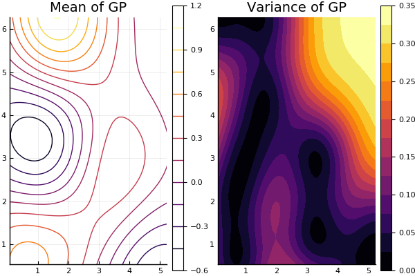

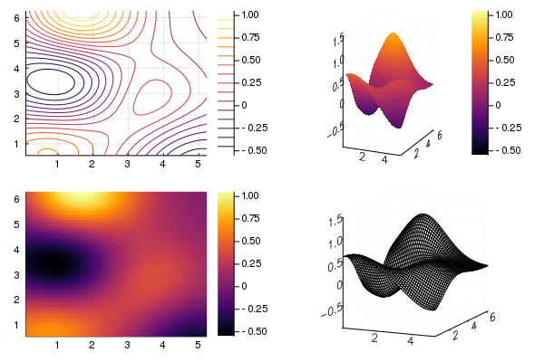
png

Plots.jl has recipes for different types of two-dimensional plots including heatmaps, surfaces, contours and wireframes. The user can select the type of plot using the seriestype keyword, or the appropriate function name:

gr() # use GR backend to allow wireframe plot
p1 = contour(gp2)
p2 = surface(gp2)
p3 = heatmap(gp2)
p4 = wireframe(gp2)
plot(p1, p2, p3, p4; fmt=:png)

png