Binary classification

The package is designed to handle models of the following general form

where $\mathbf{y}=(y_1,y_2,\ldots,y_n) \in \mathcal{Y}$ and $\mathbf{x} \in \mathcal{X}$ are the observations and covariates, respectively, and $f_i:=f(\mathbf{x}_i)$ is the latent function which we model with a Gaussian process prior. We assume that the responses $\mathbf{y}$ are independent and identically distributed and as a result the likelihood $p(\mathbf{y} \ | \ \mathbf{f}, \theta)$, can be factorized over the observations.

In the case where the observations are Gaussian distributed, the marginal likelihood and predictive distribution can be derived analytically. See the Regression documentation for an illustration.

In this example we show how the GP Monte Carlo function can be used for supervised learning classification. We use the Crab dataset from the R package MASS. In this dataset we are interested in predicting whether a crab is of colour form blue or orange. Our aim is to perform a Bayesian analysis and calculate the posterior distribution of the latent GP function $\mathbf{f}$ and model parameters $\theta$ from the training data $\{\mathbf{X}, \mathbf{y}\}$.

using GaussianProcesses, RDatasets
import Distributions:Normal
using Random

Random.seed!(113355)

crabs = dataset("MASS","crabs");              # load the data
crabs = crabs[shuffle(1:size(crabs)[1]), :];  # shuffle the data

train = crabs[1:div(end,2),:];

y = Array{Bool}(undef,size(train)[1]);       # response
y[train[:,:Sp].=="B"].=0;                      # convert characters to booleans
y[train[:,:Sp].=="O"].=1;

X = convert(Matrix,train[:,4:end]);          # predictors

We assume a zero mean GP with a Matern 3/2 kernel. We use the automatic relevance determination (ARD) kernel to allow each dimension of the predictor variables to have a different length scale. As this is binary classifcation, we use the Bernoulli likelihood,

where $\Phi: \mathbb{R} \rightarrow [0,1]$ is the cumulative distribution function of a standard Gaussian and acts as a squash function that maps the GP function to the interval [0,1], giving the probability that $y_i=1$.

Note that BernLik requires the observations to be of type Bool and unlike some likelihood functions (e.g. student-t) does not contain any parameters to be set at initialisation.

#Select mean, kernel and likelihood function
mZero = MeanZero();                # Zero mean function
kern = Matern(3/2,zeros(5),0.0);   # Matern 3/2 ARD kernel (note that hyperparameters are on the log scale)
lik = BernLik();                   # Bernoulli likelihood for binary data {0,1}

We fit the GP using the general GP function. This function is a shorthand for the GPA function which is used to generate approximations of the latent function when the likelihood is non-Gaussian.

gp = GP(X',y,mZero,kern,lik)      # Fit the Gaussian process model

GP Approximate object:
  Dim = 5
  Number of observations = 100
  Mean function:
    Type: MeanZero, Params: Float64[]
  Kernel:
    Type: Mat32Ard{Float64}, Params: [-0.0, -0.0, -0.0, -0.0, -0.0, 0.0]
  Likelihood:
    Type: BernLik, Params: Any[]
  Input observations =
[16.2 11.2 … 11.6 18.5; 13.3 10.0 … 9.1 14.6; … ; 41.7 26.9 … 28.4 42.0; 15.4 9.4 … 10.4 16.6]
  Output observations = Bool[false, false, false, false, true, true, false, true, true, true  …  false, true, false, false, false, true, false, false, false, true]
  Log-posterior = -161.209

We assign Normal priors from the Distributions package to each of the Matern kernel parameters. If the mean and likelihood function also contained parameters, then we could set these priors in the same using gp.m and gp.lik in place of gp.k, respectively.

set_priors!(gp.kernel,[Normal(0.0,2.0) for i in 1:6])

6-element Array{Normal{Float64},1}:
 Normal{Float64}(μ=0.0, σ=2.0)
 Normal{Float64}(μ=0.0, σ=2.0)
 Normal{Float64}(μ=0.0, σ=2.0)
 Normal{Float64}(μ=0.0, σ=2.0)
 Normal{Float64}(μ=0.0, σ=2.0)
 Normal{Float64}(μ=0.0, σ=2.0)

Samples of the latent function $f,\theta \ | \ X,y$ are drawn using MCMC sampling. By default, the mcmc function uses the Hamiltonian Monte Carlo algorithm. Unless defined, the default settings for the MCMC sampler are: 1,000 iterations with no burn-in phase or thinning of the Markov chain.

samples = mcmc(gp; nIter=10000, burn=1000, thin=10);

Number of iterations = 10000, Thinning = 10, Burn-in = 1000
Step size = 0.100000, Average number of leapfrog steps = 10.015100
Number of function calls: 100152
Acceptance rate: 0.087600

We test the predictive accuracy of the fitted model against a hold-out dataset

test = crabs[div(end,2)+1:end,:];          # select test data

yTest = Array{Bool}(undef,size(test)[1]);   # test response data
yTest[test[:,:Sp].=="B"].=0;                  # convert characters to booleans
yTest[test[:,:Sp].=="O"].=1;

xTest = convert(Matrix,test[:,4:end]);

Using the posterior samples $\{f^{(i)},\theta^{(i)}\}_{i=1}^N$ from $p(f,\theta \ | \ X,y)$ we can make predictions $\hat{y}$ using the predict_y function to sample predictions conditional on the MCMC samples.

ymean = Array{Float64}(undef,size(samples,2),size(xTest,1));

for i in 1:size(samples,2)
    set_params!(gp,samples[:,i])
    update_target!(gp)
    ymean[i,:] = predict_y(gp,xTest')[1]
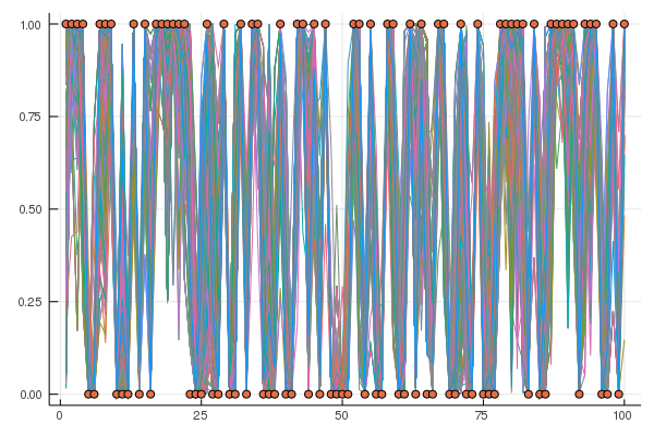
end

For each of the posterior samples we plot the predicted observation $\hat{y}$ (given as lines) and overlay the true observations from the held-out data (circles).

using Plots
gr()

plot(ymean',leg=false,html_output_format=:png)
scatter!(yTest)