Worked Example: Logistic Regression
Jack Baker
In this example we use the package to infer the bias and coefficients in a logistic regression model using stochastic gradient Langevin Dynamics with control variates. We assume we have data \(\mathbf x_1, \dots, \mathbf x_N\) and response variables \(y_1, \dots, y_N\) with likelihood \[ p(\mathbf X, \mathbf y | \beta, \beta_0 ) = \prod_{i=1}^N \left[ \frac{1}{1+e^{-\beta_0 + \mathbf x_i \beta}} \right]^{y_i} \left[ 1 - \frac{1}{1+e^{-\beta_0 + \mathbf x_i \beta}} \right]^{1-y_i} \]
First let’s load in the data, we will use the cover type dataset commonly used to benchmark classification models. We use the dataset from LIBSVM, which transforms the problem from multiclass to binary. The covertype dataset can be downloaded using the sgmcmc function getDataset as follows:
library(sgmcmc)
# Download and load covertype dataset
covertype = getDataset("covertype")
First we’ll remove about 10000 observations from the original dataset to form a test set, this will be used to check the validity of the algorithm. Then we’ll separate out the response variable y and the explanatory variables X. The response variable is the first column in the dataset.
set.seed(13)
testObservations = sample(nrow(covertype), 10^4)
testSet = covertype[testObservations,]
X = covertype[-c(testObservations),2:ncol(covertype)]
y = covertype[-c(testObservations),1]
dataset = list( "X" = X, "y" = y )
In the last line we defined the dataset as it will be input to the relevant sgmcmc function. A lot of the inputs to functions in sgmcmc are defined as lists. This improves flexibility by enabling models to be specified with multiple parameters, datasets and allows separate tuning constants to be set for each parameter. We assume that observations are always accessed on the first dimension of each object, i.e. the point \(x_i\) is located at X[i,] rather than X[,i]. Similarly the observation \(i\) from a 3d object Y would be located at Y[i,,].
Now we want to set the starting values and shapes for our parameters. We can see from the likelihood equation we have two parameters, the bias \(\beta_0\) and the coefficients \(\beta\). We’ll just set these to start from zero. Similar to the data, these are just a list with the relevant names.
# Get the dimension of X, needed to set shape of params$beta
d = ncol(dataset$X)
params = list( "bias" = 0, "beta" = matrix( rep( 0, d ), nrow = d ) )
Now we’ll define the functions logLik and logPrior. It should now become clear why the list names come in handy. The function logLik should take two parameters as input: params and dataset. These parameters will be lists with the same names as those you defined for params and dataset earlier. There is one difference though, the objects in the lists will have automatically been converted to TensorFlow objects for you. The params list will contain TensorFlow tensor variables; the dataset list will contain TensorFlow placeholders. The logLik function should take these lists as input and return the value of the log likelihood as a tensor at point params given data dataset. The function should do this using TensorFlow operations, as this allows the gradient to be automatically calculated; it also allows the wide range of distribution objects as well as matrix operations that TensorFlow provides to be taken advantage of. A tutorial of TensorFlow for R is beyond the scope of this article, for more details we refer the reader to the website of TensorFlow for R.
Specifying the logLik and logPrior functions regularly requires specifying specific distributions. TensorFlow already has a number of distributions implemented in the TensorFlow Probability package. All of the distributions implemented in TensorFlow Probability are located in tf$distributions, a list is given on the TensorFlow Probability website. More complex distributions can be specified by coding up the logLik and logPrior functions by hand, examples of this, as well as using various distribution functions, are given in the other tutorials. With this in place we can define the logLik function as follows
logLik = function(params, dataset) {
    yEstimated = 1 / (1 + tf$exp( - tf$squeeze(params$bias + tf$matmul(dataset$X, params$beta))))
    logLik = tf$reduce_sum(dataset$y * tf$log(yEstimated) + (1 - dataset$y) * tf$log(1 - yEstimated))
    return(logLik)
}
Next we want to define our log-prior density, we assume each \(\beta_i\) has an independent Laplace prior distribution, with location 0 and scale 1, so that \(\log p( \beta ) = - \sum_{i=0}^d | \beta_i|\). Similar to the log-likelihood function, the log-prior density is defined as a function with input params. In our case the definition is
logPrior = function(params) {
    logPrior = - (tf$reduce_sum(tf$abs(params$beta)) + tf$reduce_sum(tf$abs(params$bias)))
    return(logPrior)
}
Finally, we’ll set the stepsize parameters for the algorithm, along with the minibatch size. sgldcv relies on two stepsize parameters, one for the optimization step and one for the MCMC step. To allow stepsizes to be set for different parameters, the form of the stepsizes for the MCMC will be lists with names corresponding to each of the names in params. The optimization step will just be one value as the stepsize is automatically tuned
stepsizesMCMC = list("beta" = 5e-6, "bias" = 5e-6)
stepsizesOptimization = 5e-6
Alternatively, we can simply use the shortcut stepsizesMCMC = 2e-5 which would set the stepsizes for each parameter to 2e-5. The optimization step is performed using the TensorFlow AdamOptimizer.
Now we can run our SGLD-CV algorithm using the function sgldcv from the sgmcmc package, which returns a list of Markov chains for each parameter as output. Use the argument verbose = FALSE to hide the output of the function. To make the results reproducible we’ll set the seed to 13. As the dataset size is quite large, we’ll change the minibatchSize from its default 0.01 * N to 500. To allow a small 1000 iteration burn-in we’ll set the number of iterations to be 11000
output = sgldcv(logLik, dataset, params, stepsizesMCMC, stepsizesOptimization, logPrior = logPrior,
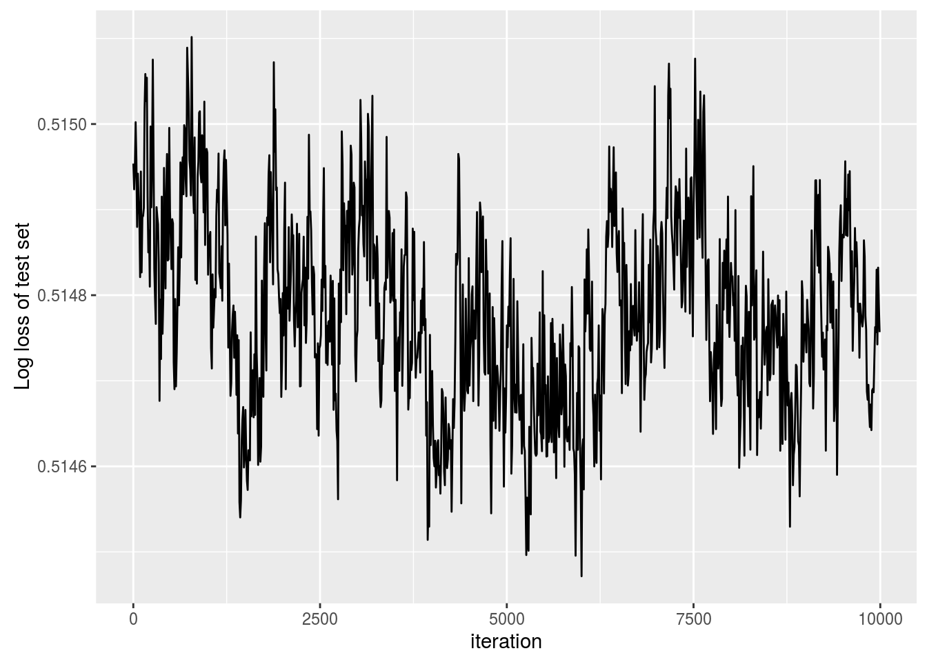
minibatchSize = 500, nIters = 11000, verbose = FALSE, seed = 13 ) A common performance measure for a classifier is the log loss. To check the algorithm converged, we’ll plot the log loss of the data from our test set every 10 iterations. Let \[\hat \pi_i^{(j)} := \frac{1}{1 + \exp\left[-\beta_0^{(j)} - \mathbf x_i \beta^{(j)}\right]},\] here \(\hat \pi_i^{(j)}\) denotes the probability that the \(j^{\text{th}}\) iteration of our MCMC chain assigned to observation \(i\) is in our test set. Define our test set by \(T\), the log loss is given by \[A := \frac{1}{|T|} \sum_{y_i \in T} \left[ y_i \log \hat \pi_i^{(j)} + (1 - y_i) \log(1 - \hat \pi_i^{(j)}) \right]\]
To check convergence, we’ll plot the log loss every 10 iterations as follows
yTest = testSet[,1]
XTest = testSet[,2:ncol(testSet)]
# Remove burn-in
output$bias = output$bias[-c(1:1000)]
output$beta = output$beta[-c(1:1000),,]
iterations = seq(from = 1, to = 10^4, by = 10)
logLoss = rep(0, length(iterations))
# Calculate log loss every 10 iterations
for ( iter in 1:length(iterations) ) {
    j = iterations[iter]
    # Get parameters at iteration j
    beta0_j = output$bias[j]
    beta_j = output$beta[j,]
    for ( i in 1:length(yTest) ) {
        pihat_ij = 1 / (1 + exp(- beta0_j - sum(XTest[i,] * beta_j)))
        y_i = yTest[i]
        # Calculate log loss at current test set point
        LogPred_curr = - (y_i * log(pihat_ij) + (1 - y_i) * log(1 - pihat_ij))
        logLoss[iter] = logLoss[iter] + 1 / length(yTest) * LogPred_curr
    }
}
library(ggplot2)
plotFrame = data.frame("iteration" = iterations, "logLoss" = logLoss)
ggplot(plotFrame, aes(x = iteration, y = logLoss)) +
    geom_line() +
    ylab("Log loss of test set")