Worked Example: Simulate from a Gaussian Mixture
Jack Baker
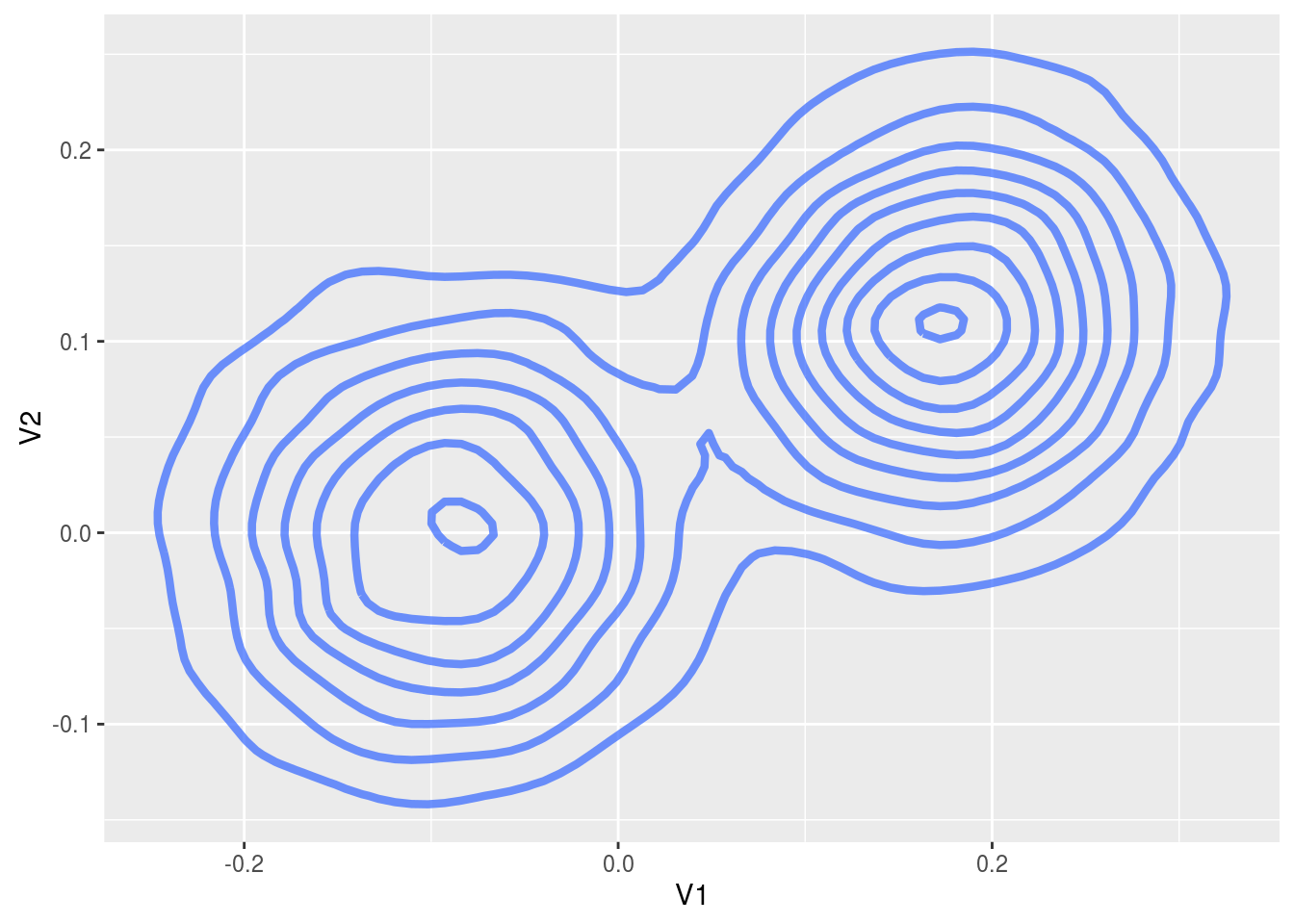
In this example we use the package to infer the modes of a bimodal, 2d Gaussian using stochastic gradient Hamiltonian Monte Carlo. So we assume we have independent and identically distributed data \(x_1, \dots, x_N\) with \(X_i | \theta \sim 0.5 N( \theta_1, I_2 ) + 0.5 N( \theta_2, I_2 )\), and we want to infer \(\theta_1\) and \(\theta_2\).
First, let’s simulate the data with the following code, we set \(N\) to be \(10^4\)
library(sgmcmc)
library(MASS)
# Declare number of observations
N = 10^4
# Set locations of two modes, theta1 and theta2
theta1 = c( 0, 0 )
theta2 = c( 0.1, 0.1 )
# Allocate observations to each component
set.seed(13)
z = sample( 2, N, replace = TRUE, prob = c( 0.5, 0.5 ) )
# Predeclare data matrix
X = matrix( rep( NA, 2*N ), ncol = 2 )
# Simulate each observation depending on the component its been allocated
for ( i in 1:N ) {
    if ( z[i] == 1 ) {
        X[i,] = mvrnorm( 1, theta1, diag(2) )
    } else {
        X[i,] = mvrnorm( 1, theta2, diag(2) )
    }
}
dataset = list("X" = X)
In the last line we defined the dataset as it will be input to the relevant sgmcmc function. A lot of the inputs to functions in sgmcmc are defined as lists. This improves flexibility by enabling models to be specified with multiple parameters, datasets and allows separate tuning constants to be set for each parameter. We assume that observations are always accessed on the first dimension of each object, i.e. the point \(x_i\) is located at X[i,] rather than X[,i]. Similarly the observation \(i\) from a 3d object Y would be located at Y[i,,].
The parameters are declared very similarly, but this time the value associated with each entry is its starting point. We have two parameters theta1 and theta2, which we’ll just start from the true values for the sake of demonstration purposes
params = list( "theta1" = c( 0, 0 ), "theta2" = c( 0.1, 0.1 ) )Now we’ll define the functions logLik and logPrior. It should now become clear why the list names come in handy. The function logLik should take two parameters as input: params and dataset. These parameters will be lists with the same names as those you defined for params and dataset earlier. There is one difference though, the objects in the lists will have automatically been converted to TensorFlow objects for you. The params list will contain TensorFlow tensor variables; the dataset list will contain TensorFlow placeholders. The logLik function should take these lists as input and return the value of the log likelihood as a tensor at point params given data dataset. The function should do this using TensorFlow operations, as this allows the gradient to be automatically calculated; it also allows the wide range of distribution objects as well as matrix operations that TensorFlow provides to be taken advantage of. A tutorial of TensorFlow for R is beyond the scope of this article, for more details we refer the reader to the website of TensorFlow for R.
Specifying the logLik and logPrior functions regularly requires specifying specific distributions. TensorFlow already has a number of distributions implemented in the TensorFlow Probability package. All of the distributions implemented in TensorFlow Probability are located in tf$distributions, a list is given on the TensorFlow Probability website. More complex distributions can be specified by coding up the logLik and logPrior functions by hand, examples of this, as well as using various distribution functions, are given in the other tutorials. With this in place we can define the log-likelihood function logLik as follows
logLik = function( params, dataset ) {
    # Declare Sigma (assumed known)
    SigmaDiag = c(1, 1)
    # Declare distribution of each component
    component1 = tf$distributions$MultivariateNormalDiag( params$theta1, SigmaDiag )
    component2 = tf$distributions$MultivariateNormalDiag( params$theta2, SigmaDiag )
    # Declare allocation probabilities of each component
    probs = tf$distributions$Categorical(c(0.5,0.5))
    # Declare full mixture distribution given components and allocation probabilities
    distn = tf$distributions$Mixture(probs, list(component1, component2))
    # Declare log likelihood
    logLik = tf$reduce_sum( distn$log_prob(dataset$X) )
    return( logLik )
}
So this function basically states that our log-likelihood function is \(\sum_{i=1}^N \log \left[ 0.5 \mathcal N( x_i | \theta_1, I_2 ) + 0.5 \mathcal N( x_i | \theta_2, I_2 ) \right]\), where \(\mathcal N( x | \mu, \Sigma )\) is a Gaussian density at \(x\) with mean \(\mu\) and variance \(\Sigma\). Most of the time just specifying the constants in these functions, such as SigmaDiag, as R objects will be fine. But there are sometimes issues when these constants get automatically converted to tf$float64 objects by TensorFlow rather than tf$float32. If you run into errors involving tf$float64 then force the constants to be input as tf$float32 by using SigmaDiag = tf$constant( c( 1, 1 ), dtype = tf$float32 ).
Next we want to define our log-prior density, which we assume is uninformative \(\log p( \theta ) = \log \mathcal N(\theta | 0,10I_2)\). Similar to the log-likelihood function, the log-prior density is defined as a function, but only with input params. In our case the definition is
logPrior = function( params ) {
    # Declare hyperparameters mu0 and Sigma0
    mu0 = c( 0, 0 )
    Sigma0Diag = c(10, 10)
    # Declare prior distribution
    priorDistn = tf$distributions$MultivariateNormalDiag( mu0, Sigma0Diag )
    # Declare log prior density and return
    logPrior = priorDistn$log_prob( params$theta1 ) + priorDistn$log_prob( params$theta2 )
    return( logPrior )
}
Finally we set the tuning parameters for SGHMC, this is a list with the same names as the params list you defined earlier, and values are the stepsize for that parameter.
stepsize = list( "theta1" = 2e-5, "theta2" = 2e-5 )Optionally, we can set the tuning parameter for the momentum alpha in the same way as the stepsize. But we’ll leave this along with the trajectory tuning constant L, and the minibatchSize as their defaults.
Now we can run our SGHMC algorithm using the sgmcmc function sghmc, which returns a list of Markov chains for each parameter as output. Use the argument verbose = FALSE to hide the output of the function. To make the results reproducible we’ll set the seed to 13. We’ll set the number of iterations as 11000 to allow for 1000 iterations of burn-in.
chains = sghmc( logLik, dataset, params, stepsize, logPrior = logPrior, nIters = 11000,
        verbose = FALSE, seed = 13 )
Finally, we’ll plot the results after removing burn-in
library(ggplot2)
# Remove burn in
burnIn = 10^3
chains = list( "theta1" = as.data.frame( chains$theta1[-c(1:burnIn),] ),
               "theta2" = as.data.frame( chains$theta2[-c(1:burnIn),] ) )
# Concatenate the two chains for the plot to get a picture of the whole distribution
plotData = rbind(chains$theta1, chains$theta2)
ggplot( plotData, aes( x = V1, y = V2 ) ) +
    stat_density2d( size = 1.5, alpha = 0.7 )